Single degree of freedom system with harmonic base displacement |
|
| A single degree of freedom system is subjected to a harmonic base displacement. We are interested in finding out the displacements at the top. |
 |
| The following geometrical data are available: |
- m: lumped mass of the single degree of freedom system = 0.5 Tonne.
- k: axial stiffness of the spring-type element = 200 N/mm.
- l : spring length = 500 mm.
- w : frequency of the external harmonic base displacement = 5 and then 20 rad/s.
- Amplitude of the external harmonic base displacement = 20 mm.
|
S.d.o.f. with Support Excitation |
| Create elements and assign attributes |
| Create two nodes with a distance of y=500 mm (say), and a beam element between them. Assign the spring/damper property to the beam, entering the correct value for the axial stiffness. From the attribute menu select Node Translational Mass and apply a 0.5 T mass to the top node. |
|
| Assign the harmonic excitation to the base node |
| Assign a vertical unity displacement to the base node and then specify a Factor vs Time table which describes its harmonic variation. |
| Simply follow the next steps: |
- Select Attributes Node/Restraint
- Check the Y value and specify 1 in the edit box.
- Select the top node and press Apply
|
|
|
- Now go to Table Factor vs. Time
- To insert values by using a particular function press the f(x) button.
- Now you can specify a function using the "x" unknown.
- Enter the values range and the number of sample points (for example from 0 to 3 s and from 1 to 80 sample points).
- Go to the Linear Transient Dynamic Solver.
- Select Load Tables and choose the table name you have just specified for the freedom condition.
|
|
|
- Set the time steps and any other information about the solver options.
|
Theoretical Solution - S.d.o.f. system without damping |
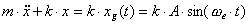
| The theoretical solution is obtained by solving the following ordinary linear, second order differential equation: |
 |
| The natural frequency of the system is given by: |
 rad/s rad/s |
| If the external and the natural frequency are equal we obtain the resonant response. In this case, the displacement of point B is harmonic but its amplitude increases linearly. Consider the case with an external frequency equal to 5 rad/s. The general solution for this case is: |
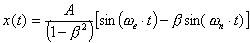 |
where,  |
|
Theoretical Solution - S.d.o.f. system with damping |
| In this case the equation describing the physical behaviour of the system is: |
 |
| with the following steady-state response: |
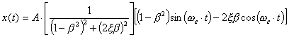 |
where,  is the damping ratio. is the damping ratio. |
To add the damping simply enter its value in the property dialog box. |
 |
|
Numerical Results |
| The Linear Transient Dynamic Solver was used to solve the models. |
|
| The Models |
  |
 |
| S.d.o.f. without damping, external frequency = 5 rad/s |
 |
| S.d.o.f. without damping, resonant response |
 |
| S.d.o.f. with damping, resonant response |
|
S.d.o.f. with non zero initial conditions |
| This example illustrates how to solve the same system of the previous example when a force is firstly applied to it and then realeased. |
|
How to build the model |
- Create the Spring/Damper element and specify its properties.
- Apply a Node Point Force at the top node.
- Specify a Table with a 1 value before the release time and 0 after that.
- Run the Linear Static Solver.
- Go to Solver/Linear Transient Dynamic.
- Specify as Initial Condition the previous linear static result file (*.lsa)
|
|
|
- Specify the Time Steps and the other solver parameters
- Press Solve
|
Theoretical Solution |
| The theoretical solution is obtained by solving the following ordinary second order differential equation: |
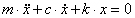 |
| with the following initial conditions: |
 and and  |
where  is the displacement at the top node because of the point load applied. is the displacement at the top node because of the point load applied. |
| If we assign c as |
 |
| the solution has the following expression: |
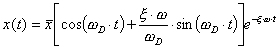 |
| where: |
 is the natural frequency of the damped system = is the natural frequency of the damped system =  |
|
Numerical Results |
| The following graph is obtained: |
 |
